MAP 6197Mathematical Introduction to Deep LearningPaper presentation

Prevalence of Neural Collapse during the terminal phase of deep learning training

Vardan Papyan, X.Y. Han, David L. Donoho

Proceedings of the National Academy of Sciences 117(40), 24652–24663, 2020 · doi:10.1073/pnas.2015509117

Presented by Thanh Bui · University of Central Florida · Fall 2026 Press → to begin · ? for controls

01MotivationAssumptions

Assumption: Deep net = feature map + linear classifier.

image \(x\in\R^d\)

Feature engineering

\(\bh=\bh_\theta(x)\)

last-layer activations \(\in\R^p\)

Classifier

\(\bW\bh+\bb\)

\(\hat y=\arg\max_c\)

\[ \hat y(\bh)=\arg\max_{c}\;\langle \bw_c,\bh\rangle + b_c, \text{ where } \bW\in\R^{C\times p},\;\bb\in\R^{C} \]

Training objective (balanced data, \(N\) examples per class)

\[ \min_{\theta,\bW,\bb}\;\sum_{c=1}^{C}\sum_{i=1}^{N} \mathcal{L}\big(\bW\bh_\theta(x_{i,c})+\bb,\;\boldsymbol{y}_c\big) \]

\(C,\ N\)number of classes; training examples per class \(x_{i,c}\)the \(i\)-th training input of class \(c\), with one-hot label \(\boldsymbol y_c\) \(\bh_{i,c}\in\R^p\)its last-layer feature \(\bh_\theta(x_{i,c})\) \(\bw_c,\ b_c\)classifier and bias of class \(c\) (row \(c\) of \(\bW\), entry \(c\) of \(\bb\))

\(\mathcal L\) is cross-entropy.

Observed Statistics

Global mean, class-means\(\bmu_G=\mean_{i,c}\bh_{i,c},\quad \bmu_c=\mean_{i}\bh_{i,c}\)
Between-class spread\(\bSigma_B=\mean_{c}(\bmu_c-\bmu_G)(\bmu_c-\bmu_G)^{\top}\)
Within-class spread\(\bSigma_W=\mean_{i,c}(\bh_{i,c}-\bmu_c)(\bh_{i,c}-\bmu_c)^{\top}\)
Centered class-means\(\bM=[\bmu_c-\bmu_G]_{c=1}^{C}\in\R^{p\times C}\)

01MotivationThe terminal phase of training · HW 2, Exercise 2.3

Training doesn’t stop at zero error.

Standard practice keeps minimizing cross-entropy after every training example is classified correctly. The paper calls this the Terminal Phase of Training (TPT).

Warm-up · HW 2, Exercise 2.3 · data \((-1,0),\,(1,1)\), no bias

\[ F(\theta)=\log\!\big(1+e^{-\theta}\big),\qquad F'(\theta)=-\tfrac{1}{1+e^{\theta}}<0 \]

Zero training error \(\iff\theta>0\), yet the loss keeps falling: \(\inf F=0\) is never attained and \(\theta_k\to\infty\).
Weight decay \(\tfrac{\lambda}{2}\theta^2\) gives a finite minimizer \(\theta^\star\). The paper trains with exactly this recipe.

The question

A deep net keeps training after zero error. What happens to its features?

Here only \(|\theta|\) can grow. A deep net can also reshape its features, and the paper finds they settle into one rigid, symmetric shape: Neural Collapse.

Weight decay

Gradient descent from θ₀ = −1.5, η = 0.5 (≤ 1/L = 4, Ex. 2.3c)

02Four collapsesOverview

Four events emerge during TPT.

NC1Within-class variability collapses: \(\bSigma_W\to\mathbf 0\)\(\tfrac1C\Tr(\bSigma_W\bSigma_B^\dagger)\) = –
NC2Class-means converge to a Simplex ETF\(\mean|\cos+\tfrac{1}{C-1}|\) = –
NC3Classifiers converge to the class-means (self-duality)\(\|\tilde\bW^\top-\tilde\bM\|_F^2\) = –
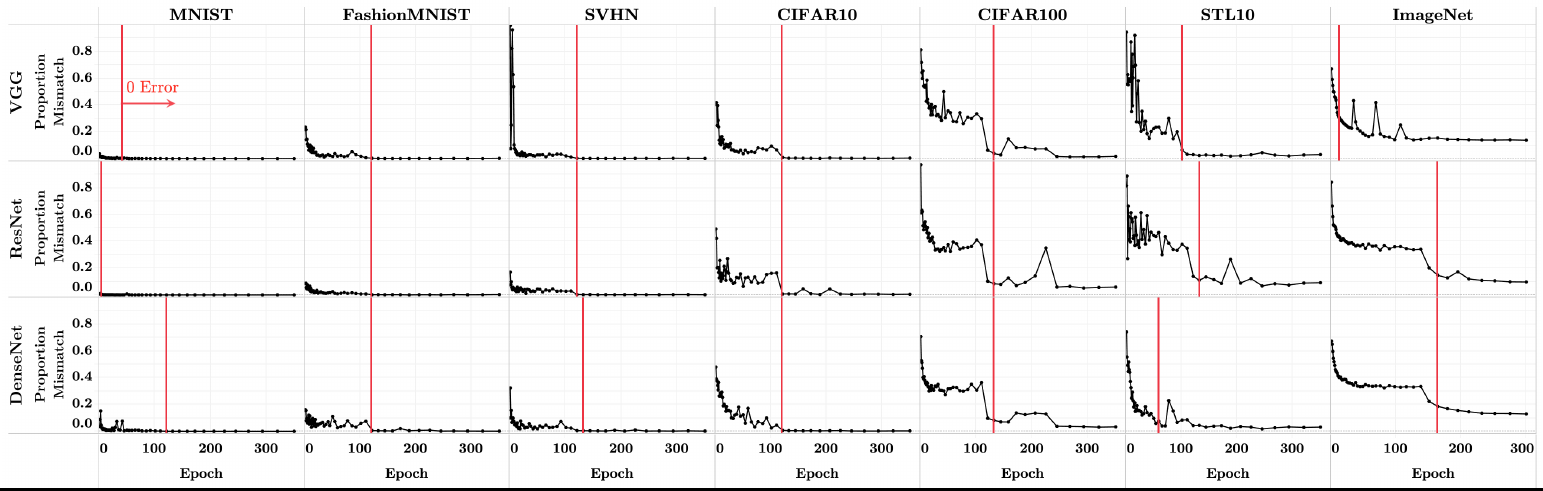
NC4Decision rule becomes nearest class-centermismatch with NCC = –

Train error = – · TPT starts at epoch –drag to rotate

An illustrative simulation in \(\R^3\) with \(C=4\), where the Simplex ETF is a regular tetrahedron. The geometry is scripted to follow NC1–NC4; every number on the left is computed live from the simulated points. The real measurements come later.

02Four collapsesDefinition · Simplex equiangular tight frame

The Simplex ETF: \(C\) vectors as far apart as possible.

Definition 1 (standard Simplex ETF)

\[ \bM^\star=\sqrt{\tfrac{C}{C-1}}\Big(\bI_C-\tfrac1C\one_C\one_C^\top\Big)\in\R^{C\times C} \]

General Simplex ETF: \(\bM=\alpha\,\bU\bM^\star\) with \(\alpha>0\) and \(\bU\in\R^{p\times C}\), \(\bU^\top\bU=\bI\) (rotation + scale).

\[ \langle\tilde\bmu_c,\tilde\bmu_{c'}\rangle=\tfrac{C}{C-1}\,\delta_{c,c'}-\tfrac{1}{C-1} \]

Equal norms and equal pairwise angles. Why \(-\tfrac1{C-1}\) is the extreme value:

\[ 0=\Big\|\sum_c\tilde\bmu_c\Big\|^2=C+\sum_{c\ne c'}\cos\angle(\bmu_c,\bmu_{c'}) \;\Rightarrow\; \overline{\cos}=-\tfrac{1}{C-1} \]

\(C=2\): 180° · \(C=3\): 120° · \(C=4\): 109.5° · \(C=10\): \(\cos=-\tfrac19\) · large \(C\): close to orthogonal

Standard basis \(e_1,e_2,e_3\)drag to rotate

Gram matrix \(\langle v_c, v_{c'}\rangle\), live

Pairwise angle

90.0°

Column norm

1.000

Construction for \(C=3\): center the basis vectors (project onto \(\one^\perp\)), then rescale by \(\sqrt{C/(C-1)}\).

02Four collapsesNC1 + NC2

Activations collapse onto a Simplex ETF.

NC1 · Variability collapse

\[ \bSigma_W\to\mathbf 0,\qquad\text{measured by }\ \tfrac1C\Tr\!\big(\bSigma_W\bSigma_B^\dagger\big)\ \text{(Fig. 6)} \]

NC1 metric (log scale)–

NC2 · Convergence to a Simplex ETF

\[ \|\bmu_c-\bmu_G\|\ \text{equal},\qquad \langle\tilde\bmu_c,\tilde\bmu_{c'}\rangle\to\tfrac{C}{C-1}\delta_{c,c'}-\tfrac{1}{C-1} \]

Max-angle · mean |cos + 1/(C−1)| (Fig. 4)–

Simulation · C = 3 in ℝ² · target angle 120°

Classes

Train activations2-σ within-class ellipseCentered class-meansSimplex ETF at the same scale

02Four collapsesNC3 + NC4

The classifier becomes nearest "neighbor".

NC3 · Self-duality: classifiers converge to the means

\[ \left\|\frac{\bW^\top}{\|\bW\|_F}-\frac{\bM}{\|\bM\|_F}\right\|_F\to0\quad\text{(Fig. 5)} \]

NC3 metric–

NC4 · Decisions simplify to nearest class-center

\[ \arg\max_{c}\,\langle\bw_c,\bh\rangle+b_c\;\to\;\arg\min_{c}\,\|\bh-\bmu_c\|_2\quad\text{(Fig. 7)} \]

Test mismatch: net vs. NCC–

Simulation · decision regions

Classes

Class-meansClassifiers \(\bw_c\) (rescaled)Test activationsNetwork decisionNCC boundaryDisagreement

NC3 and NC4 together. Press → for NC3 (this also starts the animation at 0.5×, from epoch 127, just before TPT), then → for NC4, which also brings in the decision regions and the hollow test points. The orange classifier vectors swing onto the blue class-means: weights and features end up as the same frame (self-duality, Fig. 5). Shaded regions are the network's actual linear decision, the dotted lines are the nearest-class-center (Voronoi) boundaries of the train means, and red marks where they disagree. Play: the red wedges vanish, so the network decides like NCC. The hollow test points are not collapsed, yet the two rules still agree, which is the held-out claim of Fig. 7. The Classes buttons apply here too; for C > 3 the shaded regions are a plane slice through the global mean, while red test points are judged in the full space. (≈1:20)

03WhyThree theorems

Collapse is the safest place for training to end.

Theorem 2 · squared-error loss

With features held fixed, the best last layer is a modified LDA (Webb & Lowe, 1990). Add NC1 + NC2 and it is forced to match the means (NC3) and to decide by the nearest mean (NC4).

\[ \bW=\tfrac1C\bM^{\top}\bSigma_T^{\dagger}\;\xrightarrow{\ \text{NC1, NC2}\ }\;\bW\propto\bM^{\top},\quad \hat y(\bh)=\arg\min_c\|\bh-\bmu_c\|_2 \]
Theorem 4 · cross-entropy loss

On separable features, gradient descent on cross-entropy heads to the max-margin classifier (Soudry et al., 2018). Add NC1 + NC2 and, again, NC3 + NC4 follow.

\[ \min_{\bW}\ \tfrac12\textstyle\sum_c\|\bw_c\|_2^2\ \ \text{s.t.}\ \ \langle\bw_c-\bw_{c'},\bh_{i,c}\rangle\ge1\;\xrightarrow{\ \text{NC1, NC2}\ }\;\bW\propto\bM^{\top} \]
Theorem 5 · information theory

Treat the class-means as codewords sent through small noise, \(\bh=\bmu_y+\bz\), \(\bz\sim\mathcal N(0,\sigma^2\bI)\), \(\|\bmu_c\|_2\le1\). The slowest-vanishing error is reached only by a Simplex ETF, read out by \(\bW=\bM^{\top},\ \bb=0\).

\[ \max_{\bM,\bW,\bb}\;-\lim_{\sigma\to0}\sigma^2\log P\{\hat y(\bh)\ne y\}=\frac{C}{C-1}\cdot\frac14 \]

Demo (Theorem 5): same noise on both. Left is a Simplex ETF, right is uneven; red × are mistakes. Lower σ and the uneven one falls further behind.

The paper's three theorems, one per →; the third → also brings in the noise demo. Theorem 2: take Webb and Lowe's 1990 result (with fixed features and squared-error loss, the optimal last layer is a modified LDA, W = (1/C) Mᵀ Σ_T†); add NC1 and NC2, so Σ_T = Σ_B and M has equal singular values, and W becomes proportional to Mᵀ (NC3) while argmax ⟨w_c, h⟩ + b_c turns into argmin ‖h − μ_c‖ (NC4). Theorem 4: the same conclusion for cross-entropy, starting from Soudry et al. 2018 (gradient descent on separable data goes to the max-margin classifier). So NC1 + NC2 force NC3 + NC4 under either loss. Theorem 5 explains NC2 itself: treat the class-means as codewords sent through vanishing Gaussian noise (which is what NC1 does to the features); among all codebooks with unit-norm codewords and linear decoders, the best large-deviations error exponent, C/(C−1) · 1/4, is achieved only by a Simplex ETF with W = Mᵀ, b = 0. Demo: same noise on both sides; lower σ and the uneven layout falls further behind. (Script note: the information-theory result is Theorem 5 in the paper.) (≈1:50)

04Experiment & discussionHow the experiments were run

480 networks, trained past zero error, then measured.

Data

Seven image datasets, all class-balanced: MNIST, SVHN and ImageNet are subsampled to 5000, 4600 and 600 images per class. Pixels are standardized; no data augmentation.
Networks

VGG, ResNet and DenseNet, with depth matched to each dataset (table →). Dropout is removed: batch norm in VGG, rate 0 in DenseNet.
Training

Cross-entropy, SGD with momentum 0.9, weight decay 5·10⁻⁴, batch 128, 350 epochs. Each net is trained at 25 learning rates and the one with the best final test error is kept.

ImageNet: 300 epochs, batch 256, weight decay 10⁻⁴, 10 learning rates.
Measurement

Weights are saved at selected epochs. The training images are passed through each saved net to record last-layer activations, giving the means, covariances and classifier. NC4 is checked on the test set.

TPT starts at 99.9% train accuracy (99.6% for ImageNet), allowing for mislabeled images.

Depth per dataset, ordered by difficulty as in the figures

	MNIST	Fashion- MNIST	SVHN	CIFAR 10	CIFAR 100	STL 10	Image- Net
VGG	11	11	11	13	13	13	19
ResNet	18	18	18	18	50	50	152
DenseNet	40	250	40	40	250	250	201

6datasets

×

3nets

×

25learning rates

+

30ImageNet runs

=

480models

Learning-rate schedule (ImageNet: drops at 1/2 and 3/4)

04Experiment & discussion7 datasets × 3 architectures · 480 trained models

The collapse is everywhere, and continues long after zero error.

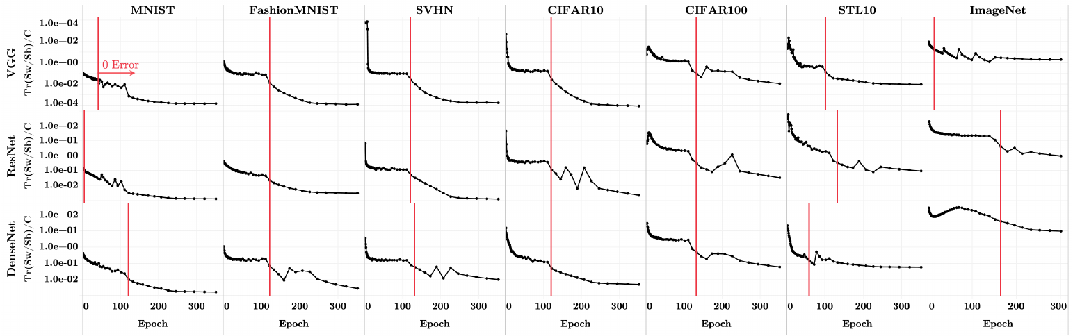
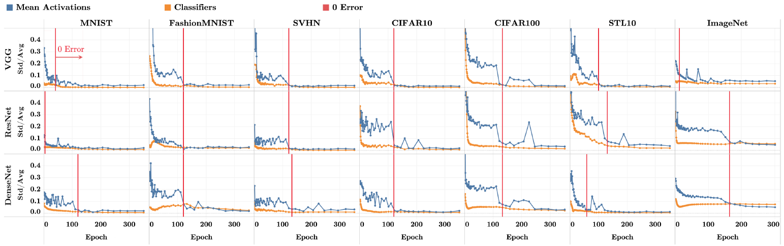
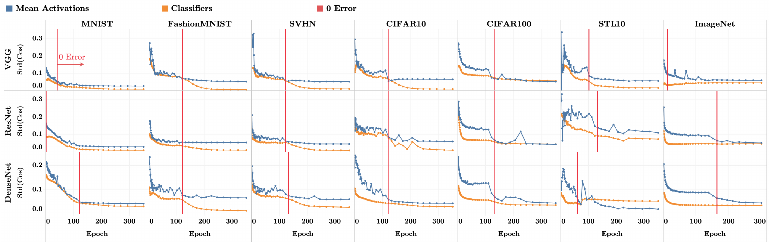
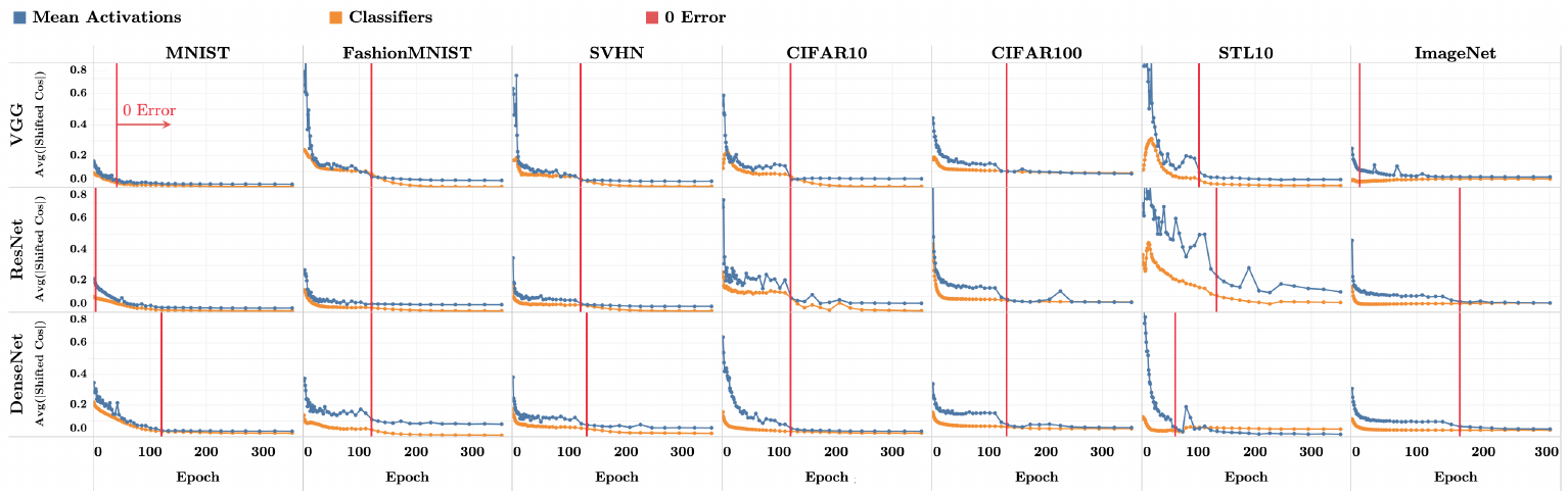
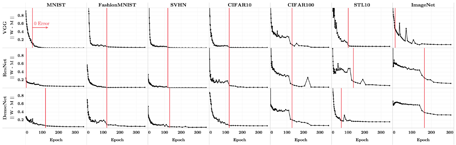
Fig. 6: Tr(Sigma_W Sigma_B^+)/C vs epoch, decreasing on log scale

Fig. 2: coefficient of variation of class-mean and classifier norms vs epoch

Fig. 3: standard deviation of pairwise cosines vs epoch

Fig. 4: average |cos + 1/(C-1)| vs epoch

Fig. 5: distance between normalized classifier and class-means vs epoch

Fig. 7: test-set disagreement between network and NCC vs epoch

↓ Lower = tighter classes\(\tfrac1C\Tr(\bSigma_W\bSigma_B^\dagger)\) on a log axis falls by several orders of magnitude for nearly every dataset–net pair. Within-class variability collapses.

↓ Lower = more equal angles\(\Std_{c\ne c'}\cos_{\bmu}(c,c')\) and \(\Std_{c\ne c'}\cos_{\bw}(c,c')\) go to zero. All pairs form equal angles.

↓ Lower = closer to the Simplex ETF angle\(\mean_{c\ne c'}|\cos+\tfrac{1}{C-1}|\to0\). The common angle is the largest possible, so it is a Simplex ETF.

↓ Lower = classifier closer to the means\(\|\bW^\top/\|\bW\|_F-\bM/\|\bM\|_F\|_F^2\) decreases. The classifier and the means converge to the same ETF.

↓ Lower = net agrees with nearest class-centerThe proportion of test points where \(\arg\max_c\langle\bw_c,\bh\rangle+b_c\ne\arg\min_c\|\bh-\bmu_c\|\) tends to zero.

How to read: rows are nets, columns are datasets ordered by difficulty. Red line = start of TPT (99.9% train acc.; 99.6% ImageNet). Blue = class-means, orange = classifiers. Press → to step through the figures.

04Experiment & discussionBenefits · Table 1 & Fig. 8

TPT also brings modest gains in accuracy and robustness.

Table 1 · test accuracy, last epoch − first zero-error epoch (percentage points)

↑ Above 0 = TPT helped · below 0 = it hurt

+0.35

median gain (pp) over 21 pairs; mean +0.50

3 of 21 decrease (red), so the gains are not universal.

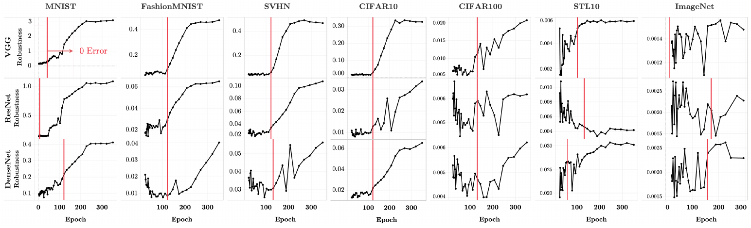
Fig. 8: robustness vs epoch increasing during TPT

Fig. 8 · adversarial robustness (DeepFool, 100 test images)

↑ Higher = harder to fool (more robust)

\[ \mean_i\,\|r(x_i)\|_2/\|x_i\|_2 \]

\(r(x_i)\) is the smallest perturbation that flips the prediction. Most of the gain happens during TPT. The median improvement is 0.0252 and the mean is 0.2452, so the mean is dominated by a few cells such as MNIST.

04Experiment & discussion Discussion

My perspective & what came next.

My perspective

Not every task wants collapse

One representation of multimodal biological data, used for several tasks

For clustering it looks good: clustering works like classification, so tight, well-separated groups help.
But the same representation also feeds other biological tasks.
There we never want different cells to share one representation: collapse erases the cell-to-cell differences those tasks need.

The next paper

Neural Collapse Under MSE Loss

Han, Papyan & Donoho · ICLR 2022 · Outstanding Paper Award

Swap cross-entropy for squared error: the same four collapses appear.
It explains how training gets there: at every moment the last layer is already the best fit to the current features, so only the features need to be followed.

They call this path the “central path”.

What if the last layer is not linear?

Collapse spreads backwards

Súkeník, Mondelli & Lampert · NeurIPS 2023

Put ReLU layers before the classifier: the earlier layers collapse too. This is deep neural collapse, and it is provably the best solution.

Proved for 2 classes.
The shape changes: after a ReLU every feature is ≥ 0, so the class-means end up at right angles instead of at the ETF angle.

TakeawayKeep training after zero error, and the last layer settles into the simplest, most noise-robust shape there is.

Press → to reveal each card, then the takeaway. My own view first, then two follow-ups. Top, my perspective: in my work one representation integrates multimodal biological data and serves several tasks. For clustering, collapse is fine, since clustering behaves like classification and tight, well-separated groups help. But the same embedding feeds other biological tasks, and there we never want different cells to end up with the same representation; collapse erases exactly the cell-to-cell differences those tasks rely on. Bottom left, the next paper by the same authors (ICLR 2022 Outstanding Paper): with squared-error loss the same four collapses appear, and they explain the route: at each moment the classifier is already the best least-squares fit to the current features, the "central path", so the dynamics reduce to the features alone. Bottom right, what changes if the last layers are not linear, from one paper (Súkeník, Mondelli & Lampert, NeurIPS 2023): with ReLU layers before the classifier, the earlier layers collapse too ("deep neural collapse"), and they prove this is the optimal solution for two classes. Because ReLU outputs are non-negative, the class-means end up orthogonal (right angles) rather than at the Simplex ETF angle. Close with the one-line takeaway. (≈1:40)

Thank youQuestions & discussion

Questions?

Online presentation can be found at bu1th4nh.github.io/presentations/ucf_fall26_map6197_neuralcollapse

References

Papyan, Han, Donoho. Prevalence of neural collapse during the terminal phase of deep learning training. PNAS 117(40), 2020.
Webb, Lowe. The optimised internal representation of multilayer classifier networks performs nonlinear discriminant analysis. Neural Networks 3, 1990.
Soudry, Hoffer, Nacson, Gunasekar, Srebro. The implicit bias of gradient descent on separable data. JMLR 19, 2018.
Han, Papyan, Donoho. Neural collapse under MSE loss: proximity to and dynamics on the central path. ICLR 2022.
Súkeník, Mondelli, Lampert. Deep neural collapse is provably optimal for the deep unconstrained features model. NeurIPS 2023.

Credits

Design inspiration: National Design Studio, ndstudio.gov
Typefaces: Cormorant Garamond and Great Vibes (Google Fonts)
Figure colors: Princess Colour Schemes, leahsmyth.github.io